Gain Statistical Insights into Your Data#
Woodwork provides methods on your DataFrames to allow you to use the typing information stored by Woodwork to better understand your data.
Follow along to learn how to use Woodwork’s statistical methods on a DataFrame of retail data while demonstrating the full capabilities of the functions.
[1]:
import pandas as pd
import numpy as np
from woodwork.demo import load_retail

df = load_retail()
df.ww
[1]:
| Physical Type | Logical Type | Semantic Tag(s) | |
|---|---|---|---|
| Column | |||
| order_product_id | category | Categorical | ['index'] |
| order_id | category | Categorical | ['category'] |
| product_id | category | Categorical | ['category'] |
| description | string | NaturalLanguage | [] |
| quantity | int64 | Integer | ['numeric'] |
| order_date | datetime64[ns] | Datetime | ['time_index'] |
| unit_price | float64 | Double | ['numeric'] |
| customer_name | category | Categorical | ['category'] |
| country | category | Categorical | ['category'] |
| total | float64 | Double | ['numeric'] |
| cancelled | bool | Boolean | [] |
DataFrame.ww.describe#
Use df.ww.describe() to calculate statistics for the columns in a DataFrame, returning the results in the format of a pandas DataFrame with the relevant calculations done for each column. Note, that both nan and (nan, nan) values contribute to nan_count for LatLong logical types
[2]:
df.ww.describe()
[2]:
| order_id | product_id | description | quantity | order_date | unit_price | customer_name | country | total | cancelled | |
|---|---|---|---|---|---|---|---|---|---|---|
| physical_type | category | category | string | int64 | datetime64[ns] | float64 | category | category | float64 | bool |
| logical_type | Categorical | Categorical | NaturalLanguage | Integer | Datetime | Double | Categorical | Categorical | Double | Boolean |
| semantic_tags | {category} | {category} | {} | {numeric} | {time_index} | {numeric} | {category} | {category} | {numeric} | {} |
| count | 401604 | 401604 | 401604 | 401604.0 | 401604 | 401604.0 | 401604 | 401604 | 401604.0 | 401604 |
| nunique | 22190 | 3684 | NaN | 436.0 | 20460 | 620.0 | 4372 | 37 | 3946.0 | NaN |
| nan_count | 0 | 0 | 0 | 0 | 0 | 0 | 0 | 0 | 0 | 0 |
| mean | NaN | NaN | NaN | 12.183273 | 2011-07-10 12:08:23.848567552 | 5.732205 | NaN | NaN | 34.012502 | NaN |
| mode | 576339 | 85123A | WHITE HANGING HEART T-LIGHT HOLDER | 1 | 2011-11-14 15:27:00 | 2.0625 | Mary Dalton | United Kingdom | 24.75 | False |
| std | NaN | NaN | NaN | 250.283037 | NaN | 115.110658 | NaN | NaN | 710.081161 | NaN |
| min | NaN | NaN | NaN | -80995.0 | 2010-12-01 08:26:00 | 0.0 | NaN | NaN | -277974.84 | NaN |
| first_quartile | NaN | NaN | NaN | 2.0 | NaN | 2.0625 | NaN | NaN | 7.0125 | NaN |
| second_quartile | NaN | NaN | NaN | 5.0 | NaN | 3.2175 | NaN | NaN | 19.305 | NaN |
| third_quartile | NaN | NaN | NaN | 12.0 | NaN | 6.1875 | NaN | NaN | 32.67 | NaN |
| max | NaN | NaN | NaN | 80995.0 | 2011-12-09 12:50:00 | 64300.5 | NaN | NaN | 277974.84 | NaN |
| num_true | NaN | NaN | NaN | NaN | NaN | NaN | NaN | NaN | NaN | 8872 |
| num_false | NaN | NaN | NaN | NaN | NaN | NaN | NaN | NaN | NaN | 392732 |
There are a couple things to note in the above dataframe:
The Woodwork index,
order_product_id, is not includedWe provide each column’s typing information according to Woodwork’s typing system
Any statistics that can’t be calculated for a column, such as
num_falseon aDatetimeare filled withNaN.Null values do not get counted in any of the calculations other than
nunique
DataFrame.ww.value_counts#
Use df.ww.value_counts() to calculate the most frequent values for each column that has category as a standard tag. This returns a dictionary where each column is associated with a sorted list of dictionaries. Each dictionary contains value and count.
[3]:
df.ww.value_counts()
[3]:
{'order_product_id': [{'value': 0, 'count': 1},
  {'value': 267744, 'count': 1},
  {'value': 267742, 'count': 1},
  {'value': 267741, 'count': 1},
  {'value': 267740, 'count': 1},
  {'value': 267739, 'count': 1},
  {'value': 267738, 'count': 1},
  {'value': 267737, 'count': 1},
  {'value': 267736, 'count': 1},
  {'value': 267735, 'count': 1}],
 'order_id': [{'value': '576339', 'count': 542},
  {'value': '579196', 'count': 533},
  {'value': '580727', 'count': 529},
  {'value': '578270', 'count': 442},
  {'value': '573576', 'count': 435},
  {'value': '567656', 'count': 421},
  {'value': '567183', 'count': 392},
  {'value': '575607', 'count': 377},
  {'value': '571441', 'count': 364},
  {'value': '570488', 'count': 353}],
 'product_id': [{'value': '85123A', 'count': 2065},
  {'value': '22423', 'count': 1894},
  {'value': '85099B', 'count': 1659},
  {'value': '47566', 'count': 1409},
  {'value': '84879', 'count': 1405},
  {'value': '20725', 'count': 1346},
  {'value': '22720', 'count': 1224},
  {'value': 'POST', 'count': 1196},
  {'value': '22197', 'count': 1110},
  {'value': '23203', 'count': 1108}],
 'customer_name': [{'value': 'Mary Dalton', 'count': 7812},
  {'value': 'Dalton Grant', 'count': 5898},
  {'value': 'Jeremy Woods', 'count': 5128},
  {'value': 'Jasmine Salazar', 'count': 4459},
  {'value': 'James Robinson', 'count': 2759},
  {'value': 'Bryce Stewart', 'count': 2478},
  {'value': 'Vanessa Sanchez', 'count': 2085},
  {'value': 'Laura Church', 'count': 1853},
  {'value': 'Kelly Alvarado', 'count': 1667},
  {'value': 'Ashley Meyer', 'count': 1640}],
 'country': [{'value': 'United Kingdom', 'count': 356728},
  {'value': 'Germany', 'count': 9480},
  {'value': 'France', 'count': 8475},
  {'value': 'EIRE', 'count': 7475},
  {'value': 'Spain', 'count': 2528},
  {'value': 'Netherlands', 'count': 2371},
  {'value': 'Belgium', 'count': 2069},
  {'value': 'Switzerland', 'count': 1877},
  {'value': 'Portugal', 'count': 1471},
  {'value': 'Australia', 'count': 1258}]}
DataFrame.ww.dependence#
df.ww.dependence calculates several dependence/correlation measures between all pairs of relevant columns. Certain types, like strings, can’t have dependence calculated.
The mutual information between columns A and B can be understood as the amount of knowledge you can have about column A if you have the values of column B. The more mutual information there is between A and B, the less uncertainty there is in A knowing B, and vice versa.
The Pearson correlation coefficient measures the linear correlation between A and B.
[4]:
df.ww.dependence(measures="all", nrows=1000)
/home/docs/checkouts/readthedocs.org/user_builds/feature-labs-inc-datatables/envs/v0.21.0/lib/python3.8/site-packages/woodwork/statistics_utils/_get_dependence_dict.py:125: UserWarning: Dropping columns ['order_id', 'customer_name'] to allow mutual information to run faster
  warnings.warn(
[4]:
| column_1 | column_2 | pearson | spearman | mutual_info | max | |
|---|---|---|---|---|---|---|
| 0 | quantity | total | 0.532443 | 0.708133 | 0.217693 | 0.708133 |
| 1 | quantity | unit_price | -0.128447 | -0.367468 | 0.086608 | -0.367468 |
| 2 | unit_price | total | 0.130113 | 0.313225 | 0.104822 | 0.313225 |
| 3 | product_id | unit_price | NaN | NaN | 0.142626 | 0.142626 |
| 4 | order_date | total | -0.024766 | -0.058553 | 0.001820 | -0.058553 |
| 5 | order_date | unit_price | -0.015619 | -0.053699 | 0.010496 | -0.053699 |
| 6 | total | cancelled | NaN | NaN | 0.030746 | 0.030746 |
| 7 | quantity | cancelled | NaN | NaN | 0.025767 | 0.025767 |
| 8 | product_id | total | NaN | NaN | 0.024799 | 0.024799 |
| 9 | quantity | country | NaN | NaN | 0.020539 | 0.020539 |
| 10 | country | total | NaN | NaN | 0.016507 | 0.016507 |
| 11 | product_id | quantity | NaN | NaN | 0.015635 | 0.015635 |
| 12 | quantity | order_date | 0.009907 | -0.003156 | 0.002659 | 0.009907 |
| 13 | country | cancelled | NaN | NaN | 0.007489 | 0.007489 |
| 14 | product_id | order_date | NaN | NaN | 0.003862 | 0.003862 |
| 15 | unit_price | country | NaN | NaN | 0.002613 | 0.002613 |
| 16 | order_date | country | NaN | NaN | -0.002411 | -0.002411 |
| 17 | product_id | country | NaN | NaN | 0.001545 | 0.001545 |
| 18 | order_date | cancelled | NaN | NaN | 0.000962 | 0.000962 |
| 19 | product_id | cancelled | NaN | NaN | -0.000172 | -0.000172 |
| 20 | unit_price | cancelled | NaN | NaN | 0.000133 | 0.000133 |
Available Parameters#
df.ww.dependence provides various parameters for tuning the dependence calculation.
measure- Which dependence measures to calculate. A list of measures can be provided to calculate multiple measures at once. Valid measure strings:“pearson”: calculates the Pearson correlation coefficient
“spearman”: calculates the Spearman correlation coefficient
“mutual_info”: calculates the mutual information between columns
“max”: calculates both Pearson and mutual information and returns max(abs(pearson), mutual) for each pair of columns
“all”: includes columns for “pearson”, “mutual”, and “max”
num_bins- In order to calculate mutual information on continuous data, Woodwork bins numeric data into categories. This parameter allows you to choose the number of bins with which to categorize data.Defaults to using 10 bins
The more bins there are, the more variety a column will have. The number of bins used should accurately portray the spread of the data.
nrows- Ifnrowsis set at a value below the number of rows in the DataFrame, that number of rows is randomly sampled from the underlying dataDefaults to using all the available rows.
Decreasing the number of rows can speed up the mutual information calculation on a DataFrame with many rows, but you should be careful that the number being sampled is large enough to accurately portray the data.
include_index- If set toTrueand an index is defined with a logical type that is valid for mutual information, the index column will be included in the mutual information output.Defaults to
False
Now that you understand the parameters, you can explore changing the number of bins. Note—this only affects numeric columns quantity and unit_price. Increase the number of bins from 10 to 50, only showing the impacted columns.
[5]:
dep_df = df.ww.dependence(measures="all", nrows=1000)
dep_df[
    dep_df["column_1"].isin(["unit_price", "quantity"])
    | dep_df["column_2"].isin(["unit_price", "quantity"])
]
/home/docs/checkouts/readthedocs.org/user_builds/feature-labs-inc-datatables/envs/v0.21.0/lib/python3.8/site-packages/woodwork/statistics_utils/_get_dependence_dict.py:125: UserWarning: Dropping columns ['order_id', 'customer_name'] to allow mutual information to run faster
  warnings.warn(
[5]:
| column_1 | column_2 | pearson | spearman | mutual_info | max | |
|---|---|---|---|---|---|---|
| 0 | quantity | total | 0.532443 | 0.708133 | 0.217693 | 0.708133 |
| 1 | quantity | unit_price | -0.128447 | -0.367468 | 0.086608 | -0.367468 |
| 2 | unit_price | total | 0.130113 | 0.313225 | 0.104822 | 0.313225 |
| 3 | product_id | unit_price | NaN | NaN | 0.142626 | 0.142626 |
| 5 | order_date | unit_price | -0.015619 | -0.053699 | 0.010496 | -0.053699 |
| 7 | quantity | cancelled | NaN | NaN | 0.025767 | 0.025767 |
| 9 | quantity | country | NaN | NaN | 0.020539 | 0.020539 |
| 11 | product_id | quantity | NaN | NaN | 0.015635 | 0.015635 |
| 12 | quantity | order_date | 0.009907 | -0.003156 | 0.002659 | 0.009907 |
| 15 | unit_price | country | NaN | NaN | 0.002613 | 0.002613 |
| 20 | unit_price | cancelled | NaN | NaN | 0.000133 | 0.000133 |
[6]:
dep_df = df.ww.dependence(measures="all", nrows=1000, num_bins=50)
dep_df[
    dep_df["column_1"].isin(["unit_price", "quantity"])
    | dep_df["column_2"].isin(["unit_price", "quantity"])
]
/home/docs/checkouts/readthedocs.org/user_builds/feature-labs-inc-datatables/envs/v0.21.0/lib/python3.8/site-packages/woodwork/statistics_utils/_get_dependence_dict.py:125: UserWarning: Dropping columns ['order_id', 'customer_name'] to allow mutual information to run faster
  warnings.warn(
[6]:
| column_1 | column_2 | pearson | spearman | mutual_info | max | |
|---|---|---|---|---|---|---|
| 0 | quantity | total | 0.532443 | 0.708133 | 0.338410 | 0.708133 |
| 1 | unit_price | total | 0.130113 | 0.313225 | 0.369177 | 0.369177 |
| 2 | quantity | unit_price | -0.128447 | -0.367468 | 0.105124 | -0.367468 |
| 3 | product_id | unit_price | NaN | NaN | 0.163247 | 0.163247 |
| 5 | order_date | unit_price | -0.015619 | -0.053699 | 0.011766 | -0.053699 |
| 8 | quantity | country | NaN | NaN | 0.024711 | 0.024711 |
| 9 | product_id | quantity | NaN | NaN | 0.019753 | 0.019753 |
| 10 | quantity | cancelled | NaN | NaN | 0.017920 | 0.017920 |
| 11 | quantity | order_date | 0.009907 | -0.003156 | 0.007075 | 0.009907 |
| 14 | unit_price | country | NaN | NaN | 0.006367 | 0.006367 |
| 19 | unit_price | cancelled | NaN | NaN | 0.000578 | 0.000578 |
In order to include the index column in the mutual information output, run the calculation with include_index=True.
[7]:
dep_df = df.ww.dependence(measures="all", nrows=1000, num_bins=50, include_index=True)
dep_df[
    dep_df["column_1"].isin(["order_product_id"])
    | dep_df["column_2"].isin(["order_product_id"])
]
/home/docs/checkouts/readthedocs.org/user_builds/feature-labs-inc-datatables/envs/v0.21.0/lib/python3.8/site-packages/woodwork/statistics_utils/_get_dependence_dict.py:125: UserWarning: Dropping columns ['order_id', 'customer_name'] to allow mutual information to run faster
  warnings.warn(
[7]:
| column_1 | column_2 | pearson | spearman | mutual_info | max | |
|---|---|---|---|---|---|---|
| 21 | order_product_id | product_id | NaN | NaN | 2.253709e-10 | 2.253709e-10 |
| 22 | order_product_id | order_date | NaN | NaN | 2.037283e-12 | 2.037283e-12 |
| 23 | order_product_id | total | NaN | NaN | 2.000378e-12 | 2.000378e-12 |
| 24 | order_product_id | quantity | NaN | NaN | 1.124831e-12 | 1.124831e-12 |
| 25 | order_product_id | unit_price | NaN | NaN | 1.095298e-12 | 1.095298e-12 |
| 26 | order_product_id | country | NaN | NaN | 2.011721e-13 | 2.011721e-13 |
| 27 | order_product_id | cancelled | NaN | NaN | 1.495745e-14 | 1.495745e-14 |
Outlier Detection with Series.ww.box_plot_dict#
One of the ways that Woodwork allows for univariate outlier detection is the IQR, or interquartile range, method. This can be done on a by-column basis using the series.ww.box_plot_dict method that identifies outliers and includes the statistical data necessary for building a box and whisker plot.
[8]:
total = df.ww["total"]
box_plot_dict = total.ww.box_plot_dict()

print("high bound: ", box_plot_dict["high_bound"])
print("low_bound: ", box_plot_dict["low_bound"])
print("quantiles: ", box_plot_dict["quantiles"])
print("number of low outliers: ", len(box_plot_dict["low_values"]))
print("number of high outliers: ", len(box_plot_dict["high_values"]))
high bound:  71.15625
low_bound:  -31.47375
quantiles:  {0.0: -277974.84, 0.25: 7.0124999999999975, 0.5: 19.305, 0.75: 32.669999999999995, 1.0: 277974.84}
number of low outliers:  1922
number of high outliers:  31016
We can see that the total column in the retail dataset has many outliers, and they are skewed more towards the top of the dataset. There are around 400K rows in the dataframe, so about 8% of all values are outliers. Let’s also look at a normally distributed column of data of the same length and see what the statistics generated for it look like.
[9]:
rnd = np.random.RandomState(33)
s = pd.Series(rnd.normal(50, 10, 401604))
s.ww.init()
box_plot_dict = s.ww.box_plot_dict()

print("high bound: ", box_plot_dict["method"])
print("high bound: ", box_plot_dict["high_bound"])
print("low_bound: ", box_plot_dict["low_bound"])
print("quantiles: ", box_plot_dict["quantiles"])
print("number of low outliers: ", len(box_plot_dict["low_values"]))
print("number of high outliers: ", len(box_plot_dict["high_values"]))
high bound:  box_plot
high bound:  77.04098
low_bound:  22.89795
quantiles:  {0.0: 4.519658918840335, 0.25: 43.20158903786463, 0.5: 49.988236390934304, 0.75: 56.73734594188448, 1.0: 95.28094989391388}
number of low outliers:  1460
number of high outliers:  1381
With the normally distributed set of data, the likelyhood of outliers is closer to what we’d expect, around .7%.
Outlier Detection with Series.ww.medcouple_dict#
Another way that Woodwork allows for univariate outlier detection is through the medcouple statistic, implemented via series.ww.medcouple_dict. Similar to series.ww.box_plot_dict, this method also returns the information necessary to build a box and whiskers plot
[10]:
total = df.ww["total"]
medcouple_dict = total.ww.medcouple_dict()

print("medcouple: ", medcouple_dict["method"])
print("medcouple: ", medcouple_dict["medcouple_stat"])
print("high bound: ", medcouple_dict["high_bound"])
print("low_bound: ", medcouple_dict["low_bound"])
print("quantiles: ", medcouple_dict["quantiles"])
print("number of low outliers: ", len(medcouple_dict["low_values"]))
print("number of high outliers: ", len(medcouple_dict["high_values"]))
medcouple:  medcouple
medcouple:  0.111
high bound:  71.40484
low_bound:  -31.22676
quantiles:  {0.0: -277974.84, 0.25: 7.0124999999999975, 0.5: 19.305, 0.75: 32.669999999999995, 1.0: 277974.84}
number of low outliers:  1928
number of high outliers:  31001
The number of outliers identified has decreased to around 7% of the rows. Additionally the direction of these outliers has changed, with more lower outliers and fewer higher outliers being identified. This is because the medcouple statistic takes into account the skewness of the distribution when determining which points are most likely to be outliers. For distributions that have a long tail, the Box Plot method might not be as appropriate. The medcouple statistic is calculated based on at most
10,000 randomly sampled observations in the column. This value can be changed within Config settings via ww.config.set_option("medcouple_sample_size", N).
[11]:
rnd = np.random.RandomState(33)
s = pd.Series(rnd.normal(50, 10, 401604))
s.ww.init()
medcouple_dict = s.ww.medcouple_dict()
print("medcouple: ", medcouple_dict["medcouple_stat"])
print("high bound: ", medcouple_dict["high_bound"])
print("low_bound: ", medcouple_dict["low_bound"])
print("quantiles: ", medcouple_dict["quantiles"])
print("number of low outliers: ", len(medcouple_dict["low_values"]))
print("number of high outliers: ", len(medcouple_dict["high_values"]))
medcouple:  -0.003
high bound:  77.04126
low_bound:  22.89823
quantiles:  {0.0: 4.519658918840335, 0.25: 43.20158903786463, 0.5: 49.988236390934304, 0.75: 56.73734594188448, 1.0: 95.28094989391388}
number of low outliers:  1460
number of high outliers:  1380
As you can see, the medcouple statistic is close to 0, which indicates a data with little to no skew. The outliers identified via the Medcouple statistic are around the same quantity as those via the Box Plot method when the data is normal.
Outlier Detection with Series.ww.get_outliers#
Knowing whether to use the box plot method or the medcouple approach can be confusing. You might not know whether a distrbiution is skewed or not, and if it is, whether its skewed enough to warrant using medcouple_dict. The method get_outliers can be used to address these issues. Running series.ww.get_outliers with the default method of best will return the outlier information based on the best approach.
This is determined by taking the medcouple statistic of a random sampling of the series. If the absolute value of the medcouple statistic of that sampling is under the default value of 0.3, then the method chosen will be box plot. If it is greater than or equal to 0.3, it will be the medcouple approach that is used (as this indicates that there is at least an average amount of skewness in the distribution).
To change this default medcouple threshold of 0.3, feel free to change the value in Config settings via ww.config.set_option("medcouple_threshold", 0.5).
Inferring Frequency from Noisy Timeseries Data#
df.ww.infer_temporal_frequencies will infer the observation frequency (daily, biweekly, yearly, etc) of each temporal column, even on noisy data. If a temporal column is predominantly of a single frequency, but is noisy in any way (ie. contains duplicate timestamps, nans, gaps, or timestamps that do not align with overall frequency), this table accessor method will provide the most likely frequency as well as information about the rows of data that do not adhere to this frequency.
Inferring Non-Noisy data#
If your timeseries data is perfect and doesn’t contain any noisy data, df.ww.infer_temporal_frequencies() will return a dictionary where the keys are the columns of each temporal column and the value is the pandas alias string.
[12]:
df = pd.DataFrame(
    {
        "idx": range(100),
        "dt1": pd.date_range("2005-01-01", periods=100, freq="H"),
        "dt2": pd.date_range("2005-01-01", periods=100, freq="B"),
    }
)
df.ww.init()
df.ww.infer_temporal_frequencies()
[12]:
{'dt1': 'H', 'dt2': 'B'}
Inferring Noisy data (Missing Values)#
If your timeseries is noisy, and you pass a debug=True flag, the returned dictionary will also include debug objects for each temporal column. This object is useful in helping you understand where in your data there is a problem.
[13]:
dt1_a = pd.date_range(end="2005-01-01 10:00:00", periods=500, freq="H")
dt1_b = pd.date_range(start="2005-01-01 15:00:00", periods=500, freq="H")


df = pd.DataFrame(
    {
        "idx": range(1000),
        "dt1": dt1_a.append(dt1_b),
    }
)
df.ww.init()

infer_dict = df.ww.infer_temporal_frequencies(debug=True)

inferred_freq, debug_object = infer_dict["dt1"]

assert inferred_freq is None

debug_object
[13]:
{'actual_range_start': '2004-12-11T15:00:00',
 'actual_range_end': '2005-01-22T10:00:00',
 'message': None,
 'estimated_freq': 'H',
 'estimated_range_start': '2004-12-11T15:00:00',
 'estimated_range_end': '2005-01-22T10:00:00',
 'duplicate_values': [],
 'missing_values': [{'dt': '2005-01-01T11:00:00', 'idx': 500, 'range': 4}],
 'extra_values': [],
 'nan_values': []}
We can see in the above example, the first element of the tuple is None because the timeseries has errors and cannot be inferred.
In the debug_object, the we can clearly see the estimated_freq is H for Hourly, as well as some extra information which we will explain below.
Debug Object Description#
The debug object contains the following information:
actual_range_start: an ISO 8601 formatted string of the observed start time
actual_range_end: an ISO 8601 formatted string of the observed end time
message: a message to describe why the frequency cannot be inferred
estimated_freq: a message to describe why the frequency cannot be inferred
estimated_range_start: an ISO 8601 formatted string of the estimated start time
estimated_range_end: an ISO 8601 formatted string of the estimated end time
duplicate_values: an array of range objects (described below) of duplicate values
missing_values: an array of range objects (described below) of missing values
extra_values: an array of range objects (described below) of extra values
nan_values: an array of range objects (described below) of nan values
A range object contains the following information:
dt: an ISO 8601 formatted string of the first timestamp in this range
idx: the index of the first timestamp in this range
for duplicates and extra values, the idx is in reference to the observed data
for missing values, the idx is in reference to the estimated data.
range: the length of this range.
This information is best understood through example below:
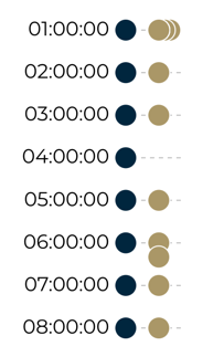
In the illustration above, you can see the expected timeseries on the left, and the observed on the right. This time series has the following errors:
Duplicate Values
“01:00:00” is duplicated twice at the observed index of 1 and 2
Missing Values
“04:00:00” is missing from estimated index 3
Extra Values
“06:20:00” is an extra value at the observed index of 7
We can recreate this example below in code. Take note that the indexes are offset by 500 since we padded the beginning of the time series with good data.
[14]:
dt_a = pd.date_range(end="2005-01-01T00:00:00.000Z", periods=500, freq="H").to_series()
dt_b = [
    "2005-01-01T01:00:00.000Z",
    "2005-01-01T01:00:00.000Z",
    "2005-01-01T01:00:00.000Z",
    "2005-01-01T02:00:00.000Z",
    "2005-01-01T03:00:00.000Z",
    "2005-01-01T05:00:00.000Z",
    "2005-01-01T06:00:00.000Z",
    "2005-01-01T06:20:00.000Z",
    "2005-01-01T07:00:00.000Z",
    "2005-01-01T08:00:00.000Z",
]
dt_b = pd.Series([pd.Timestamp(d) for d in dt_b])
dt_c = pd.date_range(
    start="2005-01-01T09:00:00.000Z", periods=500, freq="H"
).to_series()

dt = pd.concat([dt_a, dt_b, dt_c]).reset_index(drop=True).astype("datetime64[ns]")

df = pd.DataFrame({"dt": dt})
df.ww.init()
df.ww.infer_temporal_frequencies(debug=True)
/tmp/ipykernel_480/3278836014.py:19: FutureWarning: Using .astype to convert from timezone-aware dtype to timezone-naive dtype is deprecated and will raise in a future version.  Use obj.tz_localize(None) or obj.tz_convert('UTC').tz_localize(None) instead
  dt = pd.concat([dt_a, dt_b, dt_c]).reset_index(drop=True).astype("datetime64[ns]")
[14]:
{'dt': (None,
  {'actual_range_start': '2004-12-11T05:00:00',
   'actual_range_end': '2005-01-22T04:00:00',
   'message': None,
   'estimated_freq': 'H',
   'estimated_range_start': '2004-12-11T05:00:00',
   'estimated_range_end': '2005-01-22T04:00:00',
   'duplicate_values': [{'dt': '2005-01-01T01:00:00', 'idx': 501, 'range': 2}],
   'missing_values': [{'dt': '2005-01-01T04:00:00', 'idx': 503, 'range': 1}],
   'extra_values': [{'dt': '2005-01-01T06:20:00', 'idx': 507, 'range': 1}],
   'nan_values': []})}